The Texture That Won't Move

If you turn your head your nose moves with it. That is just how things work in the real world. There is a natural coherence to movement where everything on an object moves together as one. But previous GAN architectures do not have this natural coherence. The textures in the generated images are glued to the pixel grid instead of being attached to the object. So if the object moves the textures stay behind. This is called texture sticking, and once you see it you cannot unsee it.

What we are trying to achieve is a property called translational equivariance. What I mean by that is, if the input is shifted by a certain amount, the output should also be shifted by that exact same amount. The nose moves with the head. The eyes move with the face. Everything stays attached. Previous GAN generators do not have this property and the causes go deeper than you might think.

The most obvious cause is aliasing. The Nyquist-Shannon sampling theorem is a foundational theorem in signal processing that states that to perfectly reconstruct a continuous signal from its samples you must sample at a rate strictly greater than twice the highest frequency present in that signal. This threshold, half the sampling rate, is called the Nyquist limit. Aliasing occurs when a signal contains frequencies above this limit. Those excess frequencies do not just vanish. They fold back into the signal and corrupt it. In GANs specifically aliasing occurs when the generator tries to represent or sample detail at a resolution that is too low to faithfully capture it.

But aliasing is not the only problem. The network is sneakier than that. It finds multiple ways to figure out exactly where it is in absolute pixel coordinates and it exploits all of them to anchor textures to fixed positions.

Positional encoding is one of them. The generator starts from a fixed learned 4x4 tensor. As the network grows to higher resolutions it finds a way to use that base resolution as a positional reference, anchoring features to absolute pixel coordinates rather than to the object itself. Per-pixel noise inputs are another one. StyleGAN1 introduced these to let the network learn individual stochastic features like hair strands and skin pores but the model learned to use those absolute pixel positions as yet another coordinate system. And then there are image borders. The padding used in convolution operations creates detectable border patterns at the edges of feature maps and the network learns to use these borders as another positional reference, knowing where it is relative to the edge of the image.

The paper calls these unintended sources of positional information. Together with aliasing they are the full set of reasons why textures stick to pixel coordinates instead of to the object.

Now aliasing itself gets amplified by two things inside the generator. First, downsampling without proper filtering. This allows high frequency signals to leak through and corrupt the lower frequency signals at higher resolutions. Second, nonlinear activations like leaky ReLU are very aggressive towards signals. They create sharp edges which introduce high frequency components because they operate on individual pixels and produce discontinuities that the sampling rate cannot faithfully represent. Both of these compound on top of the positional information leaks to make texture sticking worse and worse as training progresses.

The result is most visible in videos generated using latent interpolation. Instead of transitioning smoothly and naturally from one frame to the next the pixels stick to screen coordinates and do not move naturally with the object. A single generated image can still look perfectly realistic. The problem only becomes obvious in motion because the textures fail to move coherently with the object across frames.

And here is the thing. Training makes this worse over time. As the network learns at higher resolutions it finds more ways to exploit these aliasing artifacts and the texture sticking builds up progressively. Nobody had rigorously solved this for GANs before StyleGAN3.

This blog is about how StyleGAN3 solved all of this, the theory behind it, my full implementation of the paper in JAX, what I redesigned and everything that broke while building it and the results I got training on a TPU v5e-8. Let's get into it!

---

Ghosts in the Pixel Grid

StyleGAN3 treats every feature map as if it were a set of discrete samples from an underlying continuous signal. Not just at the input or the output but at every single layer inside the network. That distinction turns out to matter a lot.

The paper represents the discrete signal as Z[x] and the underlying continuous signal as z(x). The two are connected through an interpolation filter and a Dirac comb III_s. The Dirac comb is just a mathematical tool that picks values from a signal at regular evenly spaced intervals, like a comb with teeth. It is used to go from the continuous signal back to the discrete signal. The interpolation filter does the opposite. It is used to go from the discrete signal to the continuous signal.

The connection between the discrete grid and the continuous signal is described by the Whittaker-Shannon interpolation formula:

Where Z[x] is the discrete feature map, z(x) is the continuous signal it represents, φ_s is the ideal interpolation filter and * denotes convolution.

There is one practical issue with this formulation. Ideal interpolation requires an infinite number of pixels in theory because the filter has influence that spreads beyond the immediate region. As a practical solution the discrete feature map is stored as a 2D array slightly larger than the s² discrete samples, large enough to capture all values that influence z(x). From this point forward the paper treats z(x) as the actual signal being operated on and Z[x] as just a convenient discrete encoding of it. In practice everything in the network is discrete but the theory reasons about the continuous signal to explain why certain operations cause aliasing.

Now upsampling and downsampling. Both of these can actually be made equivariant with proper filtering. Upsampling does not modify the continuous representation at all. Its only purpose is to increase the sampling rate to give subsequent operations more room before they hit the Nyquist limit. This is implemented practically by interleaving zeros in the discrete grid. When you interleave zeros between samples the signal now has gaps which cause the same frequency content to appear repeated at higher frequencies, like an echo in the frequency domain. Downsampling requires a lowpass filter first to remove frequencies above the Nyquist limit of the output resolution so the signal can be represented faithfully in the lower resolution grid. As long as this filtering is done correctly translation equivariance follows automatically from both operations.

So upsampling and downsampling are not the problem. They can be made equivariant. The problem is something else entirely.

The real problem is nonlinearities. Here is how the filtered nonlinearity works and this is the core contribution of the entire paper. First upsample by interleaving zeros to increase the sampling rate. Then apply a lowpass filter f_u to remove the repeating frequency copies that were created by the zero interleaving during upsampling. Then apply leaky ReLU to introduce non-linearity. But leaky ReLU operates on each pixel individually and has no idea about the continuous representation we are trying to model. It creates sharp edges which introduce very high frequencies that the discrete grid cannot represent faithfully. So after leaky ReLU we apply another lowpass filter f_d to remove all frequencies above the Nyquist limit and then we downsample to reduce the sampling rate back down.

This full pipeline is the filtered nonlinearity and it is the core of StyleGAN3. We still need non-linearity in our layers because it is important in every deep learning architecture and the filtered nonlinearity gives us exactly that while making sure the discrete feature map is fundamentally modelled as if it respected the underlying continuous signal.

One more thing before we move on. CNNs already have translational equivariance in their convolutional layers. If the input shifts, the feature maps shift in the same way. But that equivariance breaks down through operations like pooling and striding which throw away spatial information without proper filtering. StyleGAN3 pushes this much further. Every layer and operation inside the generator is redesigned to maintain strict equivariance, because if even one layer breaks it, texture sticking reappears somewhere in the pipeline.

---

Alias-Free by Design

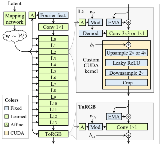
In this section I will be going through how the StyleGAN3 generator was redesigned from the StyleGAN2 generator to be an alias-free translationally equivariant network. Everything we established in the previous sections about the continuous signal, the Nyquist limit, the filtered nonlinearity and equivariance was applied practically here.

It is worth noting that the discriminator in StyleGAN3 is the exact same one from StyleGAN2. Only the generator was redesigned. This is because texture sticking is a generator side problem. The generator is what defines how features move spatially across synthesized frames so that is where the fix has to happen.

The paper introduces two configs. StyleGAN3-T for translation equivariance and StyleGAN3-R which adds rotation equivariance on top. I implemented config-T because rotation equivariance requires 1x1 convolutions throughout which limits the model's capacity and makes it harder to train. For generating cat faces translation equivariance is what matters.

So what actually changed? Almost everything in the generator.

The first change is the learned constant input. In StyleGAN2 the synthesis network starts from a fixed learned 4x4x512 tensor that the network uses as a base to build the image from. The problem is that this tensor gives the network an absolute positional anchor, a fixed coordinate system it can exploit to anchor textures to pixel coordinates. StyleGAN3 replaces this with Fourier features. Fourier features naturally define a spatially infinite feature map because frequencies are defined in the continuous domain and are not tied to a specific pixel grid. The Fourier frequencies are sampled from a circular frequency band with f_c=2 and are kept fixed over the entire course of training. They are not learned parameters. This gives the network a coordinate system that is attached to the content rather than the pixel grid. This is one of the most elegant changes in the paper because it directly addresses one of the biggest sources of texture sticking.

The per-pixel noise inputs carried over from StyleGAN1 and StyleGAN2 were also removed. Instead of the model learning the absolute position of fine stochastic details like hair strands and pores, the model inherits these naturally through the alias-free operations. This takes away yet another source of positional information that the network could exploit.

The mapping network was reduced from 8 layers to 2 layers. Path length regularization, mixing regularization and skip connections were all removed as well. These things helped keep StyleGAN2's training stable but they risked breaking equivariance and added extra compute so they all had to go. But if you remove all of these stabilization tools you still need something to keep training stable. So the underlying problem they were solving, keeping activation magnitudes stable during training, was fixed more directly with EMA variance normalization. During training the exponential moving average of the squared activation values σ² = E[x²] is tracked across all pixels and feature maps. The feature maps are then divided by √σ² to normalize their magnitude and in practice this division is baked directly into the convolution weights for efficiency. This keeps everything at a healthy magnitude throughout training while also slightly improving translational equivariance.

So now every sublayer in the generator is translationally equivariant. The learned constant that gave the network a fixed coordinate system is gone. The per-pixel noise that gave it absolute positions is gone. The padding borders are handled by adding margins around the feature maps. And every nonlinearity goes through the filtered nonlinearity pipeline to prevent aliasing from creeping in. When every layer is equivariant the whole network is equivariant and there is nothing left for textures to stick to.

Good job if you made it this far. This is where it gets real. The next section is about turning all of this theory into actual working code in JAX.

---

In JAX

I built this entire implementation from scratch in JAX. No PyTorch, no NVIDIA reference code, just the paper and raw JAX primitives. I wanted to understand every operation myself, from the filter design to the modulated convolutions to the training loop.

Why JAX specifically? I love JAX. It is a functional framework built on top of XLA which means everything compiles to optimized machine code for TPU and GPU. It forces you to think about your computation graph explicitly because there is no global state, no hidden mutation, everything is pure functional. A lot of people find this hard. I find it natural. JAX on TPU is absurdly fast and it taught me more about memory management, sharding, kernel execution, numerical precision and overflow than any textbook ever could.

I am only going to show three code blocks here. These are the operations that make StyleGAN3 what it is.

The first is the Kaiser lowpass filter design. Every layer in the generator operates at a different resolution which means every layer has a different Nyquist limit. The filter parameters have to change per layer to match. This is pure signal processing baked into the architecture before training even starts. These filters are deterministic, not learned.

import scipy.signal as sp_signal

def design_lowpass_filter(numtaps:int,cutoff:float,width:float,fs:float):

   if numtaps<=1:
       return None
   f=sp_signal.firwin(numtaps,cutoff=cutoff,width=width,fs=fs)
   return jnp.array(f,dtype=jnp.float32)

scipy.signal.firwin designs a windowed sinc filter using a Kaiser window. The cutoff frequency is the Nyquist limit of the current layer. The width controls the transition band. The number of taps is determined by filter_size multiplied by the resampling factor for that layer. None of these are hyperparameters you tune during training. They are computed automatically by compute_layer_params which builds the full per-layer schedule from the equations in Section 3 of the paper. You never have to hardcode any of it.

The second block is the filtered nonlinearity. This is the core of the entire paper and I explained the theory behind it in the previous section. Here is what it looks like in code.

def filtered_nonlinearity(x,fu,fd,up,down,
                         gain=1.4142135,slope=0.2,clamp=256.0):
   B,C,H,W=x.shape

   ## upsample by zero insertion
   if up>1:
       x_up=jnp.zeros((B,C,H*up,W*up),dtype=x.dtype)
       x_up=x_up.at[:,:,::up,::up].set(x)
       x=x_up

   ## apply upsample filter with gain=up^2 to compensate zero insertion
   if fu is not None:
       x=apply_filter_1d(x,fu,gain=float(up*up))

   ## leaky relu with gain and clamp
   x=jax.nn.leaky_relu(x,slope) * gain
   x=jnp.clip(x,-clamp,clamp)

   ## fused anti-alias filter and downsample strided conv
   if down>1 and fd is not None:
       x=apply_filter_1d_down(x,fd,down)
   elif fd is not None:
       x=apply_filter_1d(x,fd)
   elif down>1:
       x=x[:,:,::down,::down]

   return x

The code maps directly to the theory so I will not re-explain the pipeline. The things worth pointing out here are the implementation details. The gain of √2 preserves variance through leaky ReLU and the clamp at 256 prevents bfloat16 overflow which is NVIDIA's default. The apply_filter_1d_down function is an optimization I wrote that fuses the filter and downsample into a single strided depthwise convolution instead of filtering at full resolution and then discarding 75% of the computed pixels. I verified it is numerically identical with a max diff of 0.00e+00 on the forward pass.

The third block is the depthwise convolution used for filtering. This is the one that made training actually viable on TPU.

def apply_filter_1d(x,kf,gain=1.0):
   B,C,H,W=x.shape
   n=kf.shape[0]

   ## scale filter in float32 then cast to activation dtype
   kf_scaled=(kf * jnp.sqrt(jnp.float32(gain))).astype(x.dtype)

   ## horizontal pass depthwise conv tiled across C channels
   kf_h=jnp.tile(jnp.reshape(kf_scaled,(1,1,1,n)),(C,1,1,1))
   x=jax.lax.conv_general_dilated(
       lhs=x,rhs=kf_h,window_strides=(1,1),padding='SAME',
       feature_group_count=C,
       dimension_numbers=('NCHW','OIHW','NCHW'))

   ## vertical pass depthwise conv tiled across C channels
   kf_v=jnp.tile(jnp.reshape(kf_scaled,(1,1,n,1)),(C,1,1,1))
   x=jax.lax.conv_general_dilated(
       lhs=x,rhs=kf_v,window_strides=(1,1),padding='SAME',
       feature_group_count=C,
       dimension_numbers=('NCHW','OIHW','NCHW'))

   return x

The critical thing here is feature_group_count=C. My original implementation flattened the batch and channel dimensions together before the convolution. This made JAX treat it as a single large batch operation which completely bypassed the TPU MXU, the matrix multiply unit that makes TPUs fast. The MXU needs grouped matrix operations to activate and a flat B×C convolution does not give it that. Training was running at 0.18 steps per second. When I switched to feature_group_count=C which expresses the exact same operation as a grouped depthwise convolution, the MXU could finally accelerate it properly. Training jumped to 0.48 steps per second. That single change is what made training on TPU viable. This is also the same optimization that NVIDIA uses internally in their custom CUDA upfirdn2d kernel, I just arrived at it independently through JAX.

One more thing about the filter scaling line. kf_scaled computes the gain multiplication in float32 for numerical precision and then casts the result to x.dtype which is bfloat16 during training, right before the convolution. Without that explicit cast JAX silently upcasts the entire convolution to float32 which defeats the purpose of training in bfloat16. One line fix for a silent precision bleed that I did not catch for a while.

The full codebase including the generator, discriminator, mapping network, ADA augmentation pipeline, R1 regularization, EMA weight averaging, checkpoint management and the training loop is on GitHub.

---

Where Everything Went to Die

Now this is the part where I talk about everything that went wrong and how I fixed it. Building a StyleGAN3 from scratch in JAX on TPU sounds impressive until you are staring at cat shaped blobs at 4am wondering why your anti-aliasing does literally nothing. I went through a lot of pain building this and these are the three bugs that taught me the most.

Delta Filters

My original filter pipeline used 3x3 delta filters instead of proper Kaiser lowpass filters. A delta filter is essentially a filter that passes everything through unchanged. It does nothing. So my entire anti-aliasing pipeline, the core contribution of the StyleGAN3 paper, the thing that makes it different from StyleGAN2, was not active at all. Zero anti-aliasing across the entire generator.

But here is the interesting part. The model still trained and still produced faces.

GANs do not crash when anti-aliasing is missing. They just silently find workarounds using all the positional cues I talked about in the first section. The learned constant, the noise inputs, the border effects. The model was learning to generate cats by anchoring textures to pixel coordinates instead of learning proper equivariant representations. It was training as StyleGAN2 in a StyleGAN3 costume.

The root cause was actually multiple things stacked on top of each other. The filter design formula was not normalizing the transition halfwidth by the sampling rate so all the computed filters collapsed to 3 taps regardless of the layer. On top of that I was using a manual Kaiser formula instead of scipy.signal.firwin which is what NVIDIA uses internally. And on top of that, lrelu_upsampling was not set to 2. NVIDIA's filtered nonlinearity upsamples by at least 2x for every synthesis layer even when the resolution does not change between layers. Without lrelu_upsampling=2 most layers had up=1 and down=1 which means the filter either does nothing or applies a delta. The whole anti-aliasing mechanism was dead in most layers.

I only discovered this by sitting down and carefully comparing my filter outputs against what the paper specifies. The shapes were all wrong. Filters that should have been 27 to 81 taps were all 3 taps. That was the moment I realized the entire architecture was broken and everything I had trained so far was useless. Full restart.

bfloat16

This was not one bug. It was an entire category of bugs that all came from the same source. bfloat16 has 8 exponent bits and only 7 mantissa bits which gives it the same dynamic range as float32 but far less precision. On TPU v5e bfloat16 is the native dtype for the MXU so training in bfloat16 is significantly faster than float32. But that low precision creates problems everywhere.

The first problem was in the modulated convolution. The weight tensor w and the style vector s were both in bfloat16 and the demodulation step was computing means and norms in bfloat16. With 512 channels the squared values could exceed bfloat16's representable range and the norm computation would lose so much precision that the weights would silently drift to bad magnitudes over training. Nothing crashed. The outputs just got progressively worse.

The fix was pre-normalization. Before the modulated convolution I cast the weights and styles to float32 only for the norm computation, computed the scaling factor in full precision, then cast the result back to bfloat16 before multiplying.

w_f32=w.astype(jnp.float32)
s_f32=style.astype(jnp.float32)
w=w * (1.0 / jnp.sqrt(jnp.mean(w_f32**2,axis=[1,2,3],keepdims=True) + 1e-8)).astype(w.dtype)
style=style * (1.0 / jnp.sqrt(jnp.mean(s_f32**2) + 1e-8)).astype(style.dtype)

That fixed the precision but created a new problem. Once I also fixed lrelu_upsampling=2 every synthesis layer was now creating intermediate tensors at 2x resolution. With 512 channels in float32 each intermediate was about 2GB and JAX holds all of them alive during backpropagation. TPU v5e only has 16GB per chip. Training crashed during XLA compilation with RESOURCE_EXHAUSTED after trying to allocate 34GB on a 16GB device.

Two fixes. First, @nnx.remat on SynthesisLayer to recompute activations during the backward pass instead of storing them all in memory. Second, explicitly casting activations to bfloat16 after the first 1x1 convolution in the synthesis network so all downstream computation stays in bfloat16.

But even after that there was still a silent precision leak. The lowpass filter kf was stored in float32. When a float32 kernel hits a bfloat16 activation inside jax.lax.conv_general_dilated XLA silently upcasts the entire convolution to float32. My entire filter pipeline was secretly running in float32 without me knowing. This defeated the purpose of all the bfloat16 casting I had just done. The fix was one line, .astype(x.dtype) on the filter kernel right before the convolution, the same line I talked about in the previous section.

The last bfloat16 issue was the clamp at 256 in filtered_nonlinearity. Without it leaky ReLU outputs at high channel counts could theoretically exceed bfloat16's range and overflow to infinity. NVIDIA uses this same clamp in their reference code.

Step 1060

This is the one that hurt the most.

At step 1060, around 34 kimg into training, the discriminator collapsed. D loss dropped from a healthy 0.5 to 1.7 oscillation range down to 0.02 to 0.09. G loss climbed to 3 to 5. The discriminator was winning so hard that the generator was getting essentially zero useful gradient signal.

This lasted for roughly 1000 steps which is about 32 kimg of training where G was learning almost nothing.

The cause was ironic. The pre-normalization fix I added to modulated convolution for bfloat16 stability, the same fix from the previous section that solved the precision problem, also made D significantly stronger and more numerically stable. On a dataset of only 2000 images a stable discriminator can memorize the entire training set very quickly. D memorized the data faster than ADA with ada_kimg=500 could respond. By the time ADA started ramping up augmentation probability to fight back D was already dominant.

I did not intervene. I did not restart or change hyperparameters. I let it run. And D recovered naturally by around step 2000. ADA had increased augmentation enough to break D's memorization and G adapted. From step 2000 onwards training was healthy and stayed healthy all the way to 1000+ kimg.

But those 32 kimg of near-zero gradients cost something. The model trained for 180 kimg total in that early phase but only about 150 kimg of those had meaningful gradient signal. The generator's early learning was permanently delayed. The pre-normalization stabilized bfloat16 training but it also made D too powerful for a small dataset. On 200,000 images this would not have happened because D cannot memorize that much data. On 2000 images D memorized everything in 1000 steps and the augmentation pipeline was not fast enough to stop it.

---

Results

I trained on a TPU v5e-8 with a batch size of 32. The dataset was AFHQv2 cats, 2000 images at 128x128 with horizontal flips for a total effective size of 4000. The generator uses 11 synthesis layers with a channel schedule of 512 to 256, z_dim and w_dim of 512, and Fourier feature input at initial resolution 16x16. The discriminator is the same residual architecture from StyleGAN2 with minibatch standard deviation. Training ran for approximately 46,000 steps which is roughly 1488 kimg across about three weeks of sessions.

The key hyperparameters that actually mattered were g_lr=0.0025 and d_lr=0.002, r1_gamma=0.5 with lazy R1 every 16 steps, ADA with a target of 0.6 and ada_kimg=500, and EMA decay of 0.999 on the generator weights. I did not use path length regularization, mixing regularization, or skip connections. None of them. The only stabilization mechanism beyond R1 and ADA was the EMA variance normalization baked into the synthesis layers.

I want to talk about the ADA part for a second because training StyleGAN3 on 2000 images is genuinely hard. The discriminator can memorize that entire dataset in about 1000 steps if you let it, and once it does the generator stops getting useful gradients entirely. Adaptive discriminator augmentation is what makes small dataset training possible. It monitors how confident the discriminator is on real images and dynamically increases augmentation probability when D starts overfitting. NVIDIA trained on 140,000 images where the discriminator never runs out of new data to learn from. On a dataset this small ADA is not optional, it is the only reason training works at all.

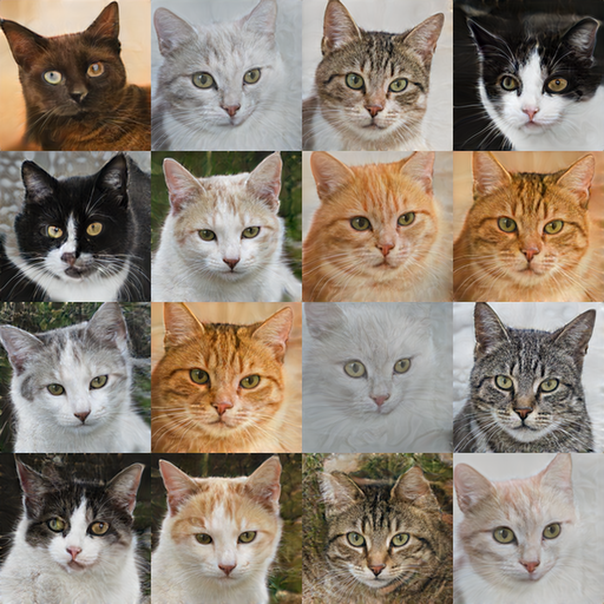
These are the generated samples from the final checkpoint using EMA weights.

The model learned distinct breed variations with visible fur textures, proper ear shapes, and realistic eye coloring with coherent pupil structure. There are black cats, tabbies, whites, calicos, and the diversity feels natural rather than forced. Whiskers are visible on several samples and the backgrounds vary rather than collapsing to a single tone which is a common failure mode when the generator gets lazy.

The latent walk is where it gets interesting. Interpolating between random points in W space produces smooth transitions between completely different cats. The fur color shifts gradually, the facial proportions morph, the ears and eyes adjust, and at no point does any frame show an obvious artifact or a discontinuous jump between two identities. The features are attached to the underlying content and not the pixel grid. When the latent code moves from one cat to another the textures actually follow. That is StyleGAN3 working as intended.

FID came out to 31.22, computed on 2000 generated samples against the real dataset using clean-fid. For context, this is on 2000 training images at 128x128. The number would be lower on a larger dataset but 31.22 on a dataset this small with a from scratch implementation is a result I am happy with.

---

Reflections

I want to talk about what this project actually looked like from my side. Not the clean code on GitHub. The real version.

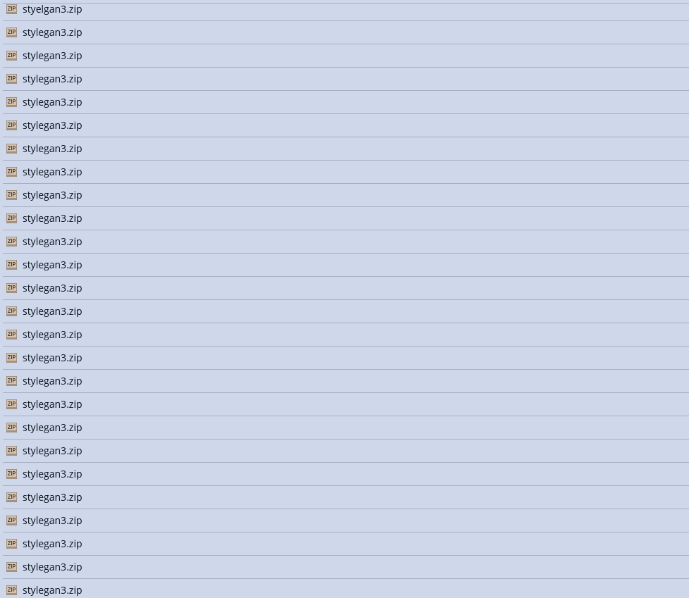
If you look at my trash folder right now it is full of stylegan3.zip files. All of them have the same name because the workflow was, change something in the code, delete the old zip, create a new one, upload it to Kaggle, run it on TPU, watch it fail, repeat. Every time I changed something I deleted the previous version and made a fresh zip. The trash just kept accumulating.

Before I wrote any code for this project I spent about two weeks reading through the GAN literature. The original GAN, DCGAN, Progressive GAN, StyleGAN1, StyleGAN2. I wanted to understand the full arc of what each paper introduced and what it was reacting to in the one before it. By the time I got to StyleGAN3 I already knew why the learned constant was a problem, why per-pixel noise leaks positional information, why AdaIN was replaced with weight demodulation. That context made the StyleGAN3 paper make sense on a level it would not have if I had just jumped straight in.

Even with that background I still read Alias-Free Generative Adversarial Networks three times. The first time I thought the filtered nonlinearity was just "add a blur after ReLU" and missed the continuous signal framework entirely. The second time I understood the Nyquist argument but could not connect it to actual code. The third time it clicked. The whole paper is one idea, treat every feature map as samples from a continuous signal and make sure nothing in the generator violates that.

The biggest thing I would do differently is the filter pipeline. I spent weeks training with delta filters, which is essentially no anti-aliasing at all, before I realized the entire core of StyleGAN3 was not active in my implementation. That whole period was wasted compute. If I had written a simple test at the start that prints filter shapes and compares them against the expected values from the paper equations I would have caught it on day one. I did not write that test because the model was training and producing faces so I assumed the filters were correct. GANs are dangerously forgiving like that. They will produce something that looks reasonable even when fundamental components are completely broken.

I also would have moved to a larger dataset sooner. 2000 images made sense for debugging but the discriminator collapse at step 1060 and most of the training instability I dealt with just would not exist on 15,000 images. I knew that and still kept running on 2000 because the iteration cycle was fast and I kept telling myself one more run.

The full codebase is at github.com/ojayballer/sg3x.

References

- Karras, T., Aittala, M., Laine, S., Harkonen, E., Hellsten, J., Lehtinen, J., & Aila, T. (2021). Alias-Free Generative Adversarial Networks. NeurIPS.
- Karras, T., Laine, S., Aittala, M., Hellsten, J., Lehtinen, J., & Aila, T. (2020). Training Generative Adversarial Networks with Limited Data. NeurIPS.
- Karras, T., Laine, S., Aittala, M., Hellsten, J., Lehtinen, J., & Aila, T. (2020). Analyzing and Improving the Image Quality of StyleGAN. CVPR.
- Karras, T., Laine, S., & Aila, T. (2019). A Style-Based Generator Architecture for Generative Adversarial Networks. CVPR.
- Goodfellow, I., et al. (2014). Generative Adversarial Nets. NeurIPS.